Benchmarking

Benchmarking napari-imagej is of interest, considering the way in which it crosses language barriers. This document serves as an initial survey of performance, in addition to being a template for further benchmarks.

To benchmark napari-imagej, we must consider how it performs relative to:

1. An equivalent Python application

2. An equivalent Java application

We consider both below, benchmarking on the goal of a simple Gaussian Blur.

This document assumes that you are running in a napari-imagej environment. For help in setting up this environment, see this page.

Data

An important part of any benchmark is the data it is run upon.

For this benchmarking procedure, we use the EmbryoCE sample from the SCIFIO Samples Repository.

This particular data sample is nice, because it is:

• Available to all

• Sufficiently large to minimize startup overhead

Unfortunately, the data is stored within separate files for each focal plane and is treated by ImageJ2 as an 8-bit image. Below, we describe the pre-processing stage necessary for the remainder of the benchmarking.

1. Configure napari-imagej settings

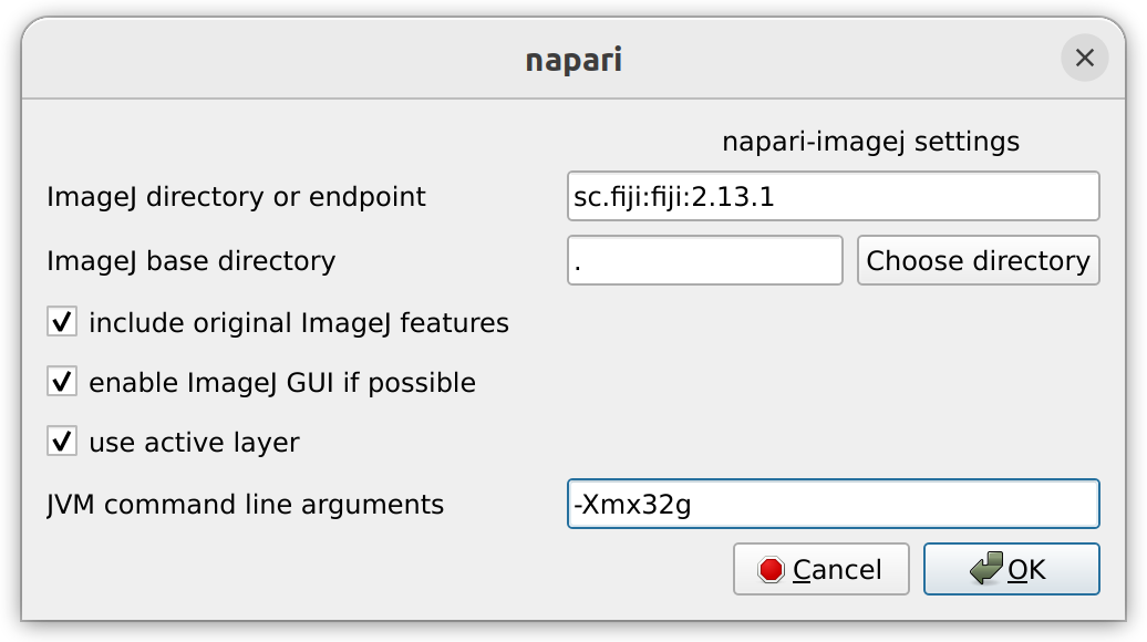
   To process EmbryoCE, we need to alter two different napari-imagej settings. For information on configuring napari-imagej, please see here.

   First, we must increase the maximum amount of RAM available to napari-imagej. This procedure provides 32GB of RAM, but the procedure can be repeated with less RAM by using fewer focal planes of EmbryoCE.

   Then, we change the backing instance of napari-imagej to sc.fiji:fiji; this gives us the Bio-Formats plugin, which will allow us to read in EmbryoCE.

   

   Recommended settings for napari-imagej benchmarking

   Once you’ve edited these settings, you’ll have to restart napari-imagej to register the changes.

2. Import EmbryoCE

   We start by using Bio-Formats to import EmbryoCE into a single input image:

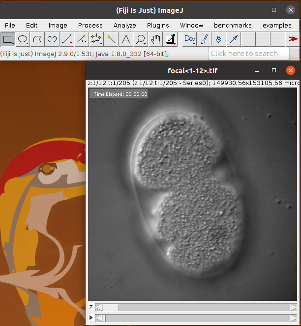
• Launch napari-imagej, and once napari-imagej is ready, launch the ImageJ GUI.

• Use Plugins -> Bio-Formats -> Bio-Formats Importer. Navigate to the downloaded EmbryoCE, and select focal1.tif. The rest of the focal planes will be automatically included.

• In Bio-Formats Import Options, do not change any settings, and click OK.

• In Bio-Formats File Stiching, change Axis 1 number of images to the number of focal planes you’d like to include. If your machine does not have 32GB of RAM, consider decreasing this number. Once finished, click OK.

  Once finished, Bio-Formats will import EmbryoCE into Fiji as a standard image.

  

  EmbryoCE loaded as a single image in Fiji

3. Convert EmbryoCE

   Many tools in the Python scientific stack automatically assume floating point math; for efficiency and speed, this is something that the ImageJ ecosystem does not do. We must convert EmbryoCE to floating-point samples to ensure uniformity.

   This is easist done with the following SciJava script, written in Python:

   convert_to_float.py

   #@ Img input
   #@output converted
   #@ OpService ops
   
   converted = ops.convert().float64(input)
   

4. Export Converted EmbryoCE

   Finally, we export the floating-point EmbryoCE as a single TIFF, again using Bio-Formats

   • Use Plugins -> Bio-Formats -> Bio-Formats Exporter and choose a suitable location, naming the image focal.tif. Click OK.

   • In Bio-Formats Exporter - Multiple Files, do not change anything, click OK.

   • In Bio-Formats Exporter Options, do not change anything, click OK.

   Once the export completes, you are ready to benchmark!

Timing in napari-imagej

Execution duration for all ImageJ2 modules is captured by napari-imagej and output to the debug logging stream (normally appearing on the console).

This means that any ImageJ2 module, including all user scripts, can be easily benchmarked by viewing these times.

To benchmark a Gaussian Blur, we use the following Python SciJava script:

gaussian_napari_imagej.py

 #@ Img input
 #@ Img output
 #@ Double sigma

 from net.imglib2.algorithm.gauss3 import Gauss3
 from net.imglib2.view import Views

 Gauss3.gauss(sigma, Views.extendMirrorSingle(input), output)

By placing this script within the ImageJ base directory (by default, the scripts directory of the napari-imagej source), the script will automatically be discovered by ImageJ2 and will be searchable using the script’s filename.

Note that this script requires a pre-allocated output image. This allows us to make use of shared memory, increasing the speed of napari-imagej.

We run the script using the following steps:

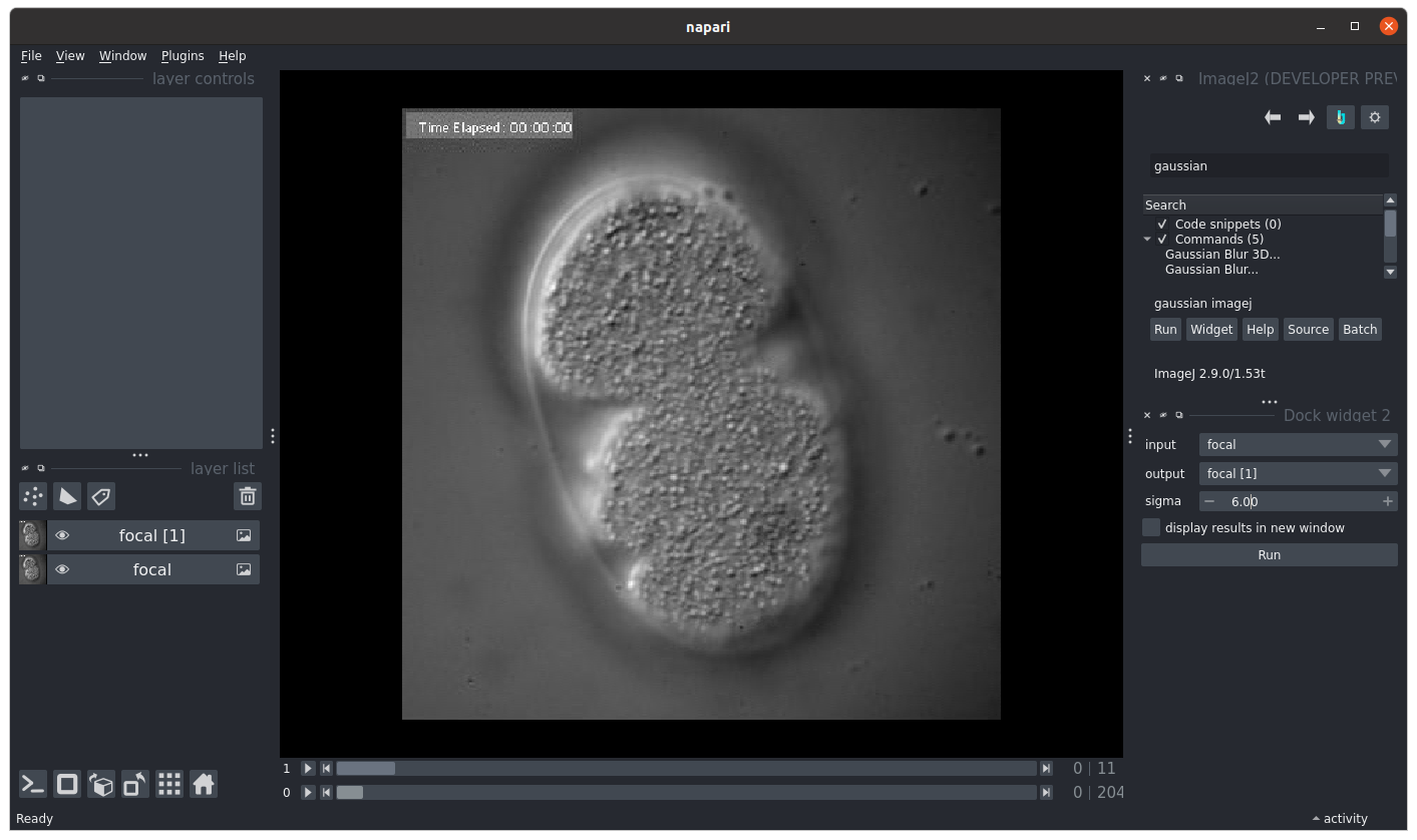
1. Launch napari-imagej

2. Load in two copies of focal.tif, the pre-processed image created above.

3. Once napari-imagej is ready, search napari-imagej for gaussian napari imagej. Launch this Module as a napari Widget with the “Widget” button.

4. In the gaussian napari imagej widget, provide

   • One copy of focal to the input parameter

   • The other copy of focal to the output parameter

   • 6.0 to the sigma parameter.

The expected napari-imagej benchmarking setup

Click “Run”, and wait for the computation to complete. Once completed, look for the following lines in the debug log:

11:10:37 DEBUG napari-imagej: Execution complete
11:10:37 DEBUG napari-imagej: Computation completed in 50.0014 seconds

Pure Java comparisons

Unfortunately, Fiji does not provide us with execution times, so the SciJava script must be modified slightly to print out its own execution time:

gaussian_fiji.py

#@ Img input
#@ Img output
#@ Double sigma

from java.lang import System
from net.imglib2.algorithm.gauss3 import Gauss3
from net.imglib2.view import Views

start = System.currentTimeMillis()

Gauss3.gauss(sigma, Views.extendMirrorSingle(input), output)

end = System.currentTimeMillis()

print("Convolution took " + str(end - start) + " milliseconds")

We run this script using the following steps:

1. Open ImageJ2. You can either use the ImageJ GUI through napari, or download an independent Fiji here.

2. Load in two copies of focal.tif, the pre-processed image created above.

3. Open the Script Editor by pressing [ with focus on the ImageJ2 menu bar.

4. Paste gaussian_fiji.py into the script editor

5. Click Run in the script editor. In the modal dialog, provide:

   • One copy of focal to the input parameter

   • The other copy of focal to the output parameter

   • 6.0 to the sigma parameter.

Click “Run”, and wait for the computation to complete. Once completed, look for the following lines in the debug log:

Started New_.py at Fri Feb 10 13:48:09 CST 2023
Convolution took 57619 milliseconds

Pure Python comparisons

To benchmark in Python, we devise a routine most similar to that performed in our prior tests. In this case, we perform a Gaussian Blur using scikit-image:

gaussian_skimage.py

from skimage.filters import gaussian
from skimage.io import imread, imsave
import timeit

path = <path to where you saved focal.tif>
img = imread(path)
sigma = 6.

num_executions = 5
times = []
for i in range(num_executions):
    duration = timeit.Timer(lambda: gaussian(img, sigma)).timeit(number=1)
    print(f"Execution {i}: {duration} seconds")
    times.append(duration)

print(f"Average execution time over {num_executions} runs: {sum(times) / len(times)}")

# save the image
out_path = "./focal_gaussed.tif"
gaussed = gaussian(img, sigma)
imsave(out_path, gaussed)

This Python script can then be run on the command line, from within the napari-imagej Mamba environment:

conda activate napari-imagej
python gauss.py

Results

To obtain suitable benchmarking results, we average each execution over 5 different runs. Each script is designed to be easily rerun: * The SciJava scripts must be manually rerun, to give the JVM time to warm up. * The pure Python script automatically reruns the computation, meaning it must only be run once to gather benchmarking data.

In the table below, we obtain the following data, running all programs on a machine with a Intel Core i7-10700 CPU, 64GB of memory, and running Ubuntu 22.04.5 LTS:

Benchmarking Data, Gaussian Blur

Trial	Scikit-Image	Fiji	napari-imagej
1	41.5903	54.564	47.197
2	41.2883	50.249	43.9305
3	41.4744	46.803	42.9653
4	41.667	45.813	43.5976
5	41.606	45.743	44.2887
Average:	41.5252	48.6344	44.39582