Using BoneJ2

Here we adapt a workflow from the BoneJ2 paper for use with napari-imagej.

napari Setup

We will install one additional napari plugin, napari-segment-blobs-and-things-with-membranes, to support this use case. Instructions for finding and installing a napari plugin are here

To install napari-segment-blobs-and-things-with-membranes, simply ensure that your napari environment is active and paste the following into your terminal:

pip install napari-segment-blobs-and-things-with-membranes

Once the plugin has been installed correctly, napari-segment-blobs-and-things-with-membranes will appear as an option within the Plugins menu of napari, and the Tools menu will be populated with the various functions of the plugin.

BoneJ2 Setup

We need to first specify the endpoint that we will use to access BoneJ2.

We can configure napari-imagej to use BoneJ2 by opening the settings dialog and changing the imagej directory or endpoint (described here). Within the napari-imagej settings dialog, paste the following into the imagej directory or endpoint field, and click OK:

sc.fiji:fiji:2.13.0+org.bonej:bonej-ops:MANAGED+org.bonej:bonej-plugins:MANAGED+org.bonej:bonej-utilities:MANAGED

Note that napari must be restarted for these changes to take effect!

Preparing and Opening the Data

We will use the same data that was used in the BoneJ2 paper. Go ahead and download umzc_378p_Apteryx_haastii_head.tif.bz2 from doi:10.6084/m9.figshare.7257179, linked directly here.

Opening Data in napari

Once you’ve unzipped the downloaded file, you can drag-and-drop the image onto napari to open it.

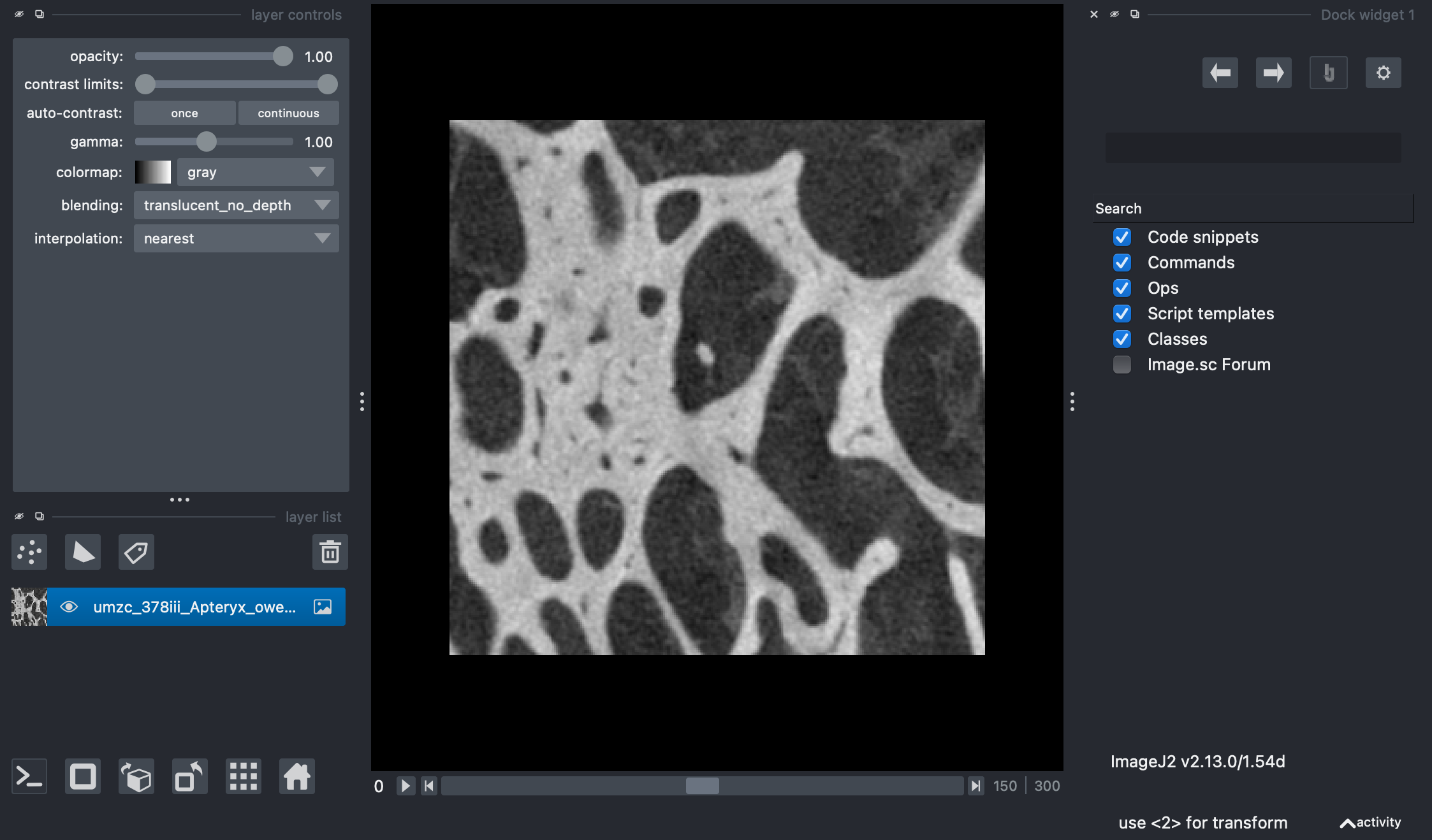
A napari viewer showing the example image that we will be working with.

Processing Data in napari with nsbatwm

Now we need to process the image.

First, we will blur the image to smooth intensity values and filter noise.

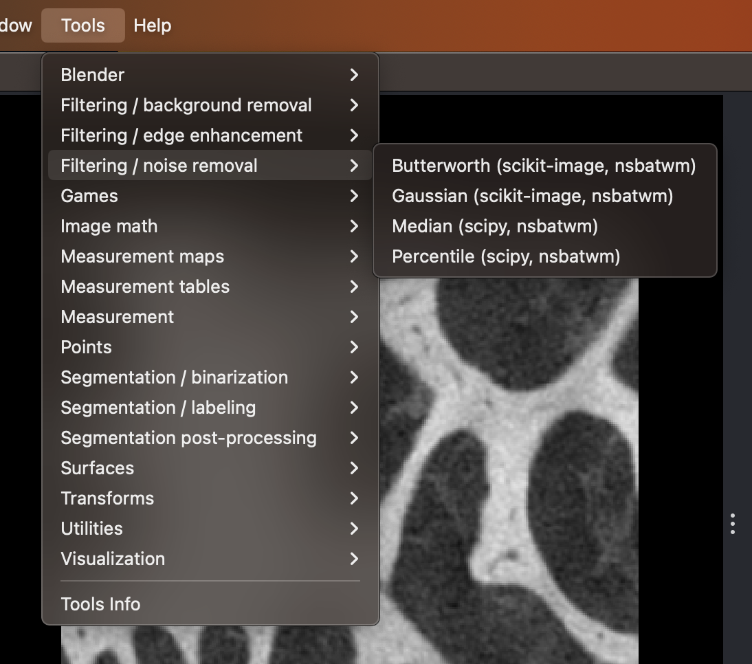
Selecting the Gaussian menu entry from the nsbatwm’s Tools menu.

1. Within napari’s menus choose: Tools > Filtering / noise removal > Gaussian (scikit image, nsbatwm)

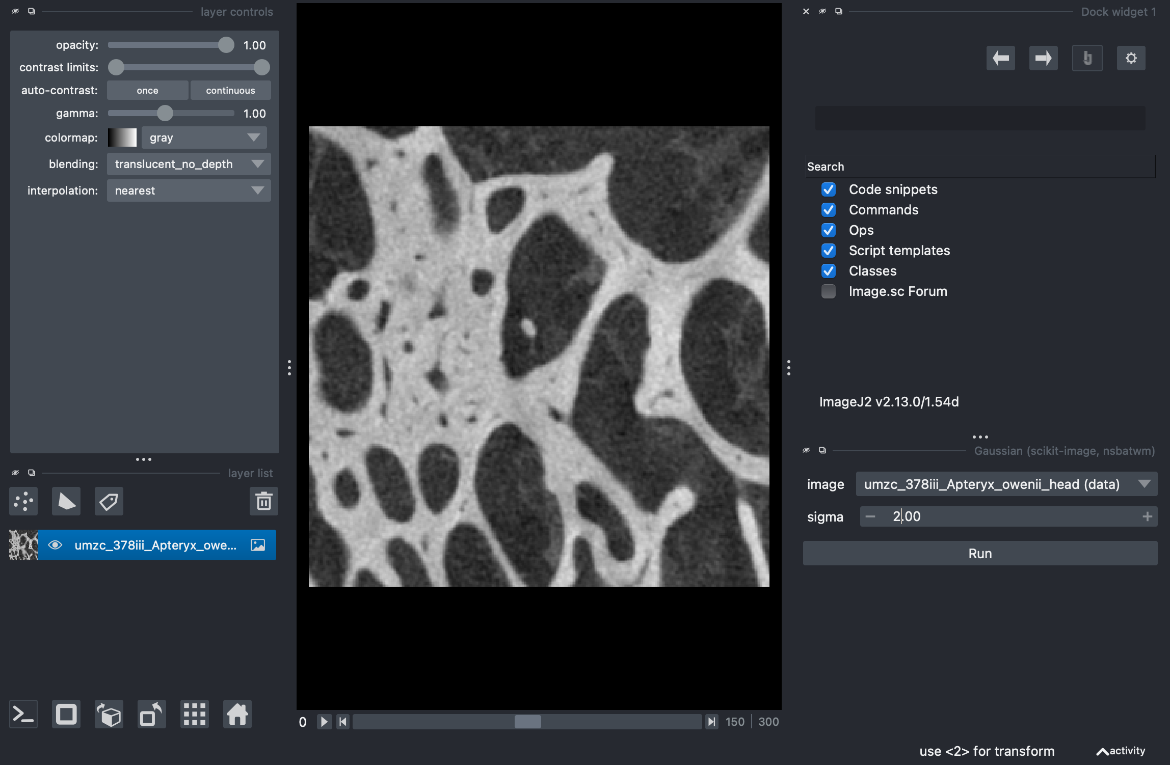
Setting the parameters for the Gaussian.

2. When the widget comes up, change the sigma value to 2 and ensure that the image layer is correctly set to the image that was opened.

3. Run the widget! When the blurring is complete, a new Image layer will appear in the napari viewer.

Now we will threshold the image to make it binary.

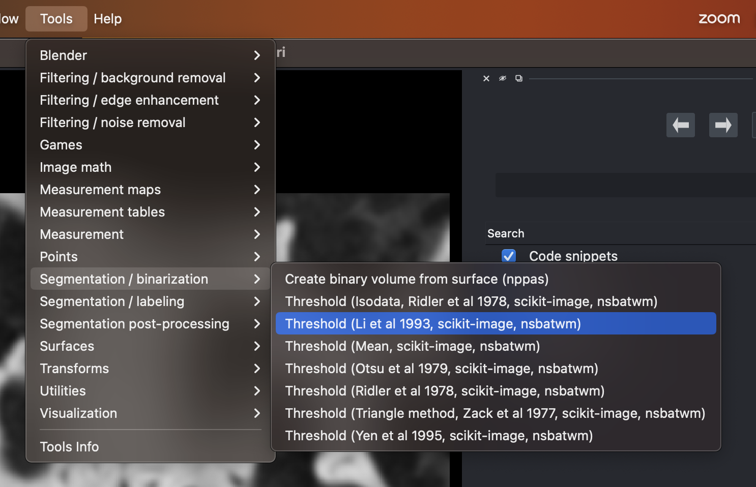
Selecting the thresholding algorithm developed by Li et al.

1. Within napari’s menus choose: Tools > Segmentation / binarization > Threshold (Li et al 1993, scikit image, nsbatwm)

2. When the widget comes up, ensure that the layer that is selected is the result of step 1.

3. Run the widget! When the thresholding is complete, a new Labels layer will appear in the napari viewer.

4. Right click on the new Labels layer and select Convert to Image. This will allow us to pass the result, now an Image layer, to BoneJ2.

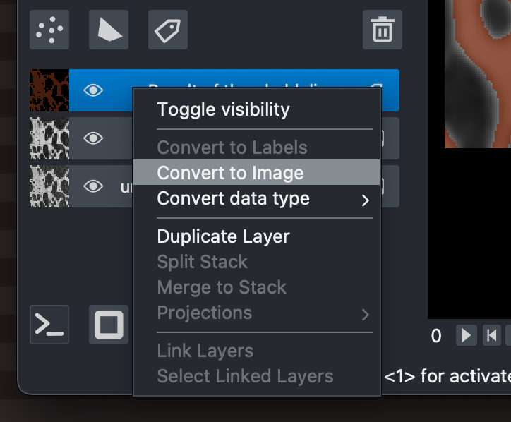
Converting the Labels layer to an Image layer for processing in BoneJ2.

Processing Data in napari with BoneJ2 and napari-imagej

Calculating the degree of anisotropy:

1. In the napari-imagej search bar type anisotropy, and select the Anisotropy Command from the search results.

2. Click Run.

3. Select the inputImage that corresponds to the theshold layer created previously.

4. Enter 1.73 as the samplingInterval.

5. Check the Recommended minimums box.

6. Click OK.

This will output the degree of anisotropy measurement for the image.

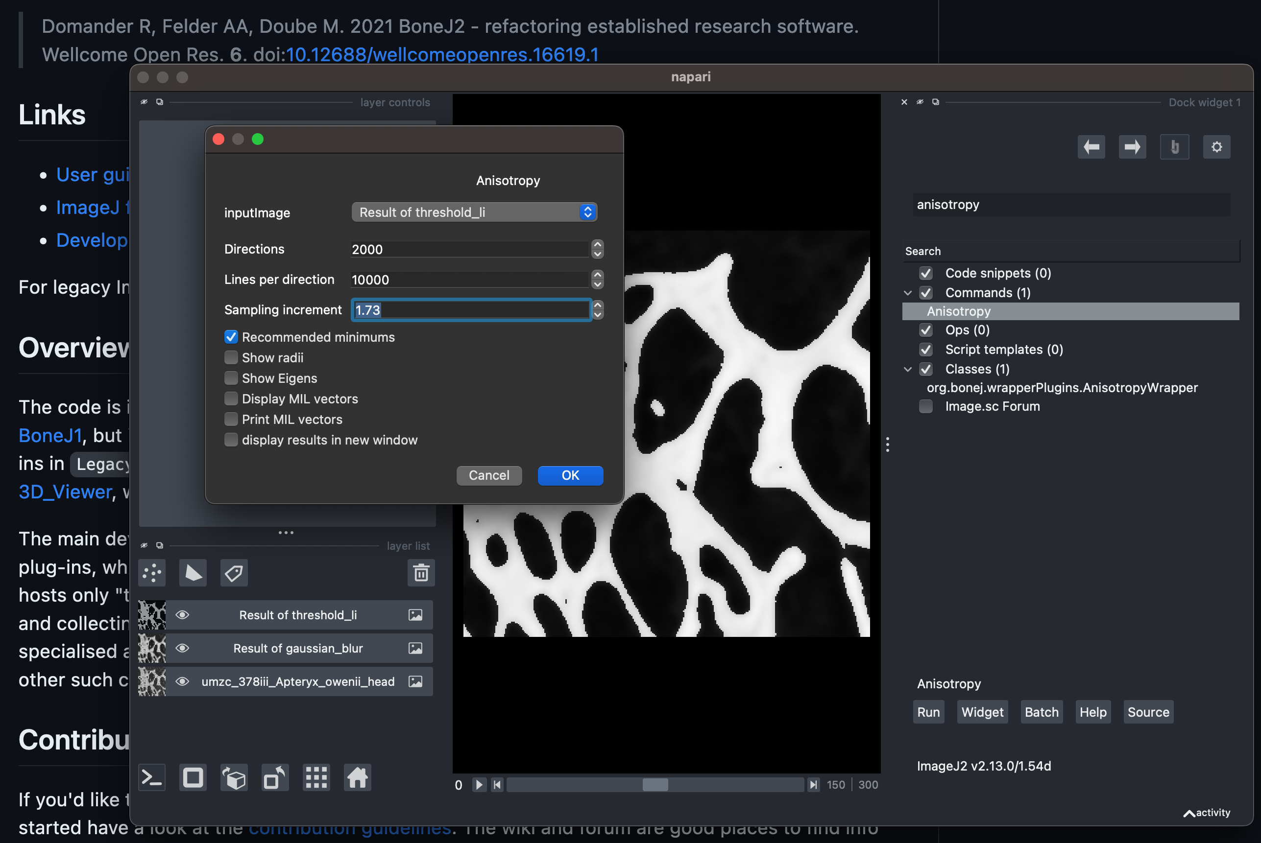
Setting the parameters of BoneJ2’s Anisotropy command.

Calculating the fractal dimension:

1. In the napari-imagej search bar type fractal dimension, and select the Fractal dimension Command from the search results.

2. Click Run.

3. Select the inputImage that corresponds to the theshold layer created previously.

4. Check the Automatic parameters box.

5. Click OK.

This will output the fractal dimension of the image.

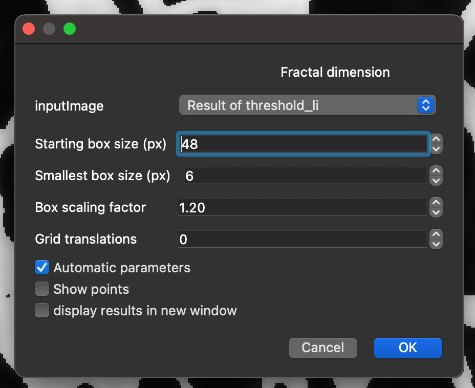
Setting the parameters of BoneJ2’s fractal dimension command.

Calculating the surface area:

1. In the napari-imagej search bar type surface area, and select the Surface area Command from the search results.

2. Click Run.

3. Select the inputImage that corresponds to the theshold layer created previously.

4. Click OK.

Note: This command may take some time, because it runs a computationally costly algorithm called “Marching Cubes” that creates a surface mesh of the image before computing the surface area. This will output the surface area of the thresholded regions.

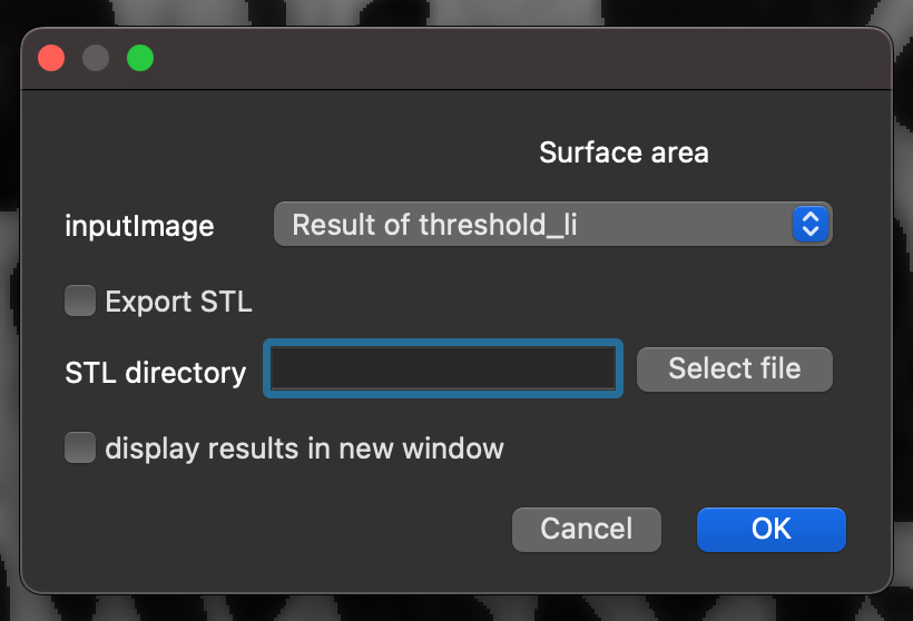
Running BoneJ2’s surface area command.

Calculating the area/volume fraction:

1. In the napari-imagej search bar type volume fraction, and select the Area/Volume fraction Command from the search results.

2. Click Run.

3. Select the inputImage that corresponds to the theshold layer created previously.

4. Click OK.

This will output the Bone Volume Fraction (BV/TV) measurement for the image.

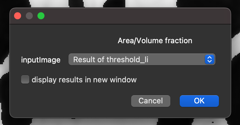
Running BoneJ2’s area/volume fraction command.

Calculating the connectivity:

1. In the napari-imagej search bar type connectivity, and select the Connectivity (Modern) Command from the search results.

2. Click Run.

3. Select the inputImage that corresponds to the theshold layer created previously.

4. Click OK.

This will output the Euler characteristic and Conn.D for the image.

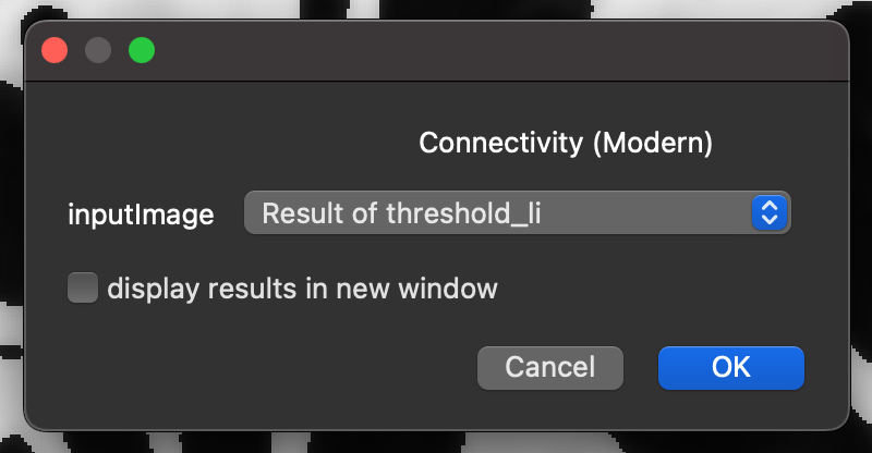
Running BoneJ2’s connectivity command.

The final measurements

We have now quantified our image with a number of methods and can use our resulting measurements in further scientific analysis!

The results table for all of the BoneJ2 measurements.